Top 20 Microsoft Excel Formulas You Must Know

Microsoft Excel is one of the most popular data analysis tools in the world. A significant number of companies depend on MS Excel for calculation, analysis and visualization of data and information. Not many are taking full advantage of this simple yet powerful tool. We made a list of Top 20 Microsoft Excel Formulas you must know to become an Excel guru.

Top 20 Microsoft Excel Formulas
You Must Know

In Microsoft Excel, a formula is an expression that calculates the values in a range of cells or cell. If you want to be more proficient in your work, improve your productivity, or impress your boss, you need to know this Microsoft Excel Formulas. We will start with some simple ones and slowly forward towards the advanced level.

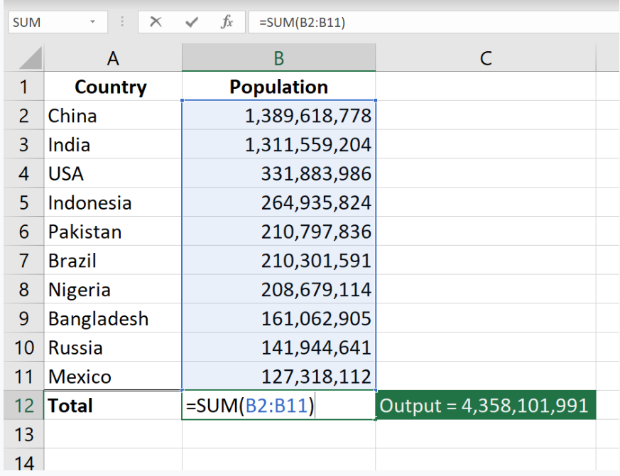
1. SUM

SUM is an excellent basic formula and one of the must know Microsoft Excel Formulas which allows you to add up numbers in different ways. Yet there are a few tricks to =SUM which provides even more functionality for adding data.

Example of the formula:

=SUM(C3:P3) – A simple way that sums the values of a selected row.

=SUM(A1:A99) – A simple selection that sums the values of a column.

=SUM(C7:C10, C21, C19:C50) – A sophisticated collection of data that sums the values from range C7 to C10. It skips the values C11 to C20 then adds from C19 to C50)

You can also turn your functions into formulas. Like,

=SUM(A1:10)/12 – Adding the values from cell A1 to cell A10 then dividing it by 12.

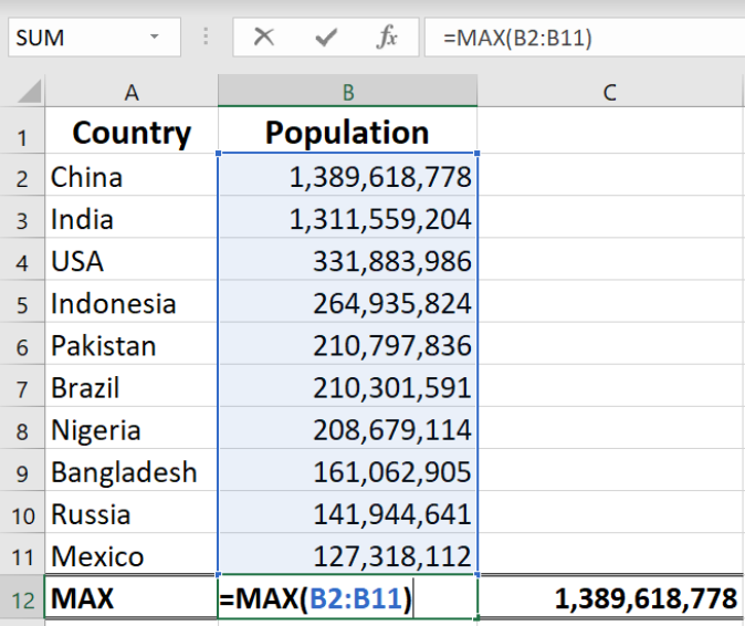
2. MAX & MIN 

If you have a spreadsheet which includes a lot of numbers, then this MAX and MIN function will help you find the maximum and minimum number in a range of values. This is another basic yet powerful Microsoft Excel Formula for finding specific number from a huge data set.

Example of the formula:

=MAX(D1:G10) – This formula finds the maximum number between column D from D1 and column G from G1 to row 10 in both columns D and G.

=MIN(D1:G10) – Similarly, it finds the minimum number between column D from D1 and column G from G1 to row 10 in both columns D and G.

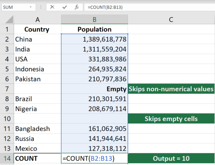
3. COUNT

The COUNT function counts all cells in a given range that contain only numeric values. It can be very handy when you extract data from another source.

Example of the formula:

=COUNT(A:A) – It counts all the values that are numerical in column A. By this formula you can also count any other columns data. It will skip the data which are not numeric.

=COUNT(A1:F1) – Now it can count numeric values of rows too.

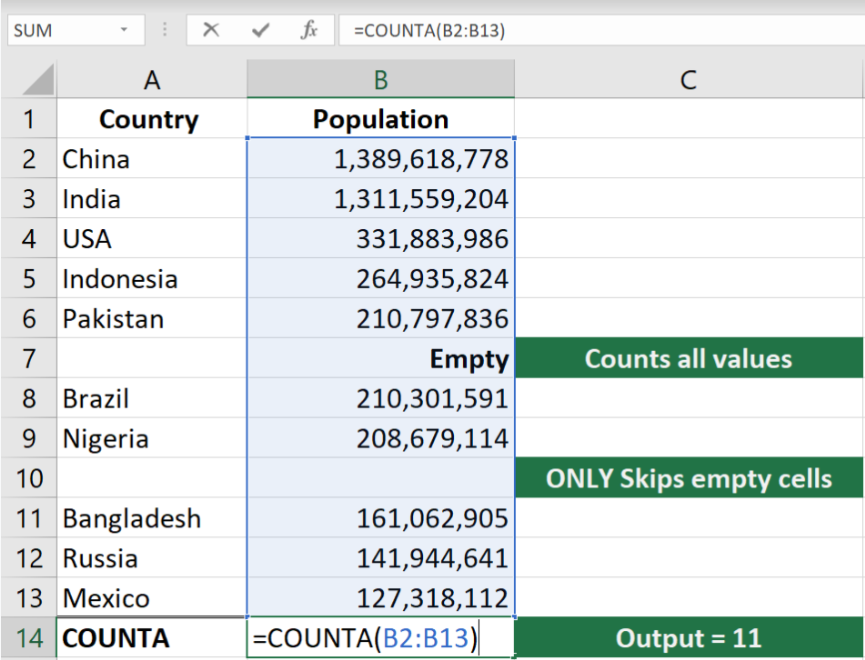
4. COUNTA

There is another COUNT function which is unique because unlike COUNT function it can count time, dates, strings, empty spaces or errors. This is another must-know Microsoft Excel Formula which is very easy to learn.

Example of the formula:

=COUNTA(D2:D13) – It counts rows 2 to 13 in column D regardless of its type. However, like COUNT, you can’t use the same formula to count rows. You need to adjust like, =COUNTA(D2:F2) which will count columns D to H.

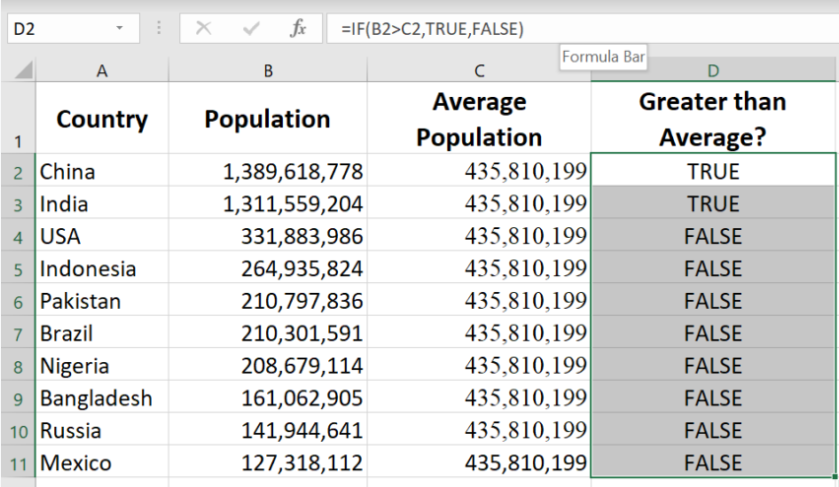
5. IF

With IF formula, Excel will tell you if a specific condition is met. This function is often used when you want to sort your data according to a given logic. And you can embed formulas and function in it too. 

Example of the formula:

=IF(A1>B2, ‘TRUE’, ‘FALSE’) – This checks if the values at A1 is greater than the value of B2. If the logic is true, let the cell value be TRUE, otherwise, FALSE.

=IF(SUM(A1:A10)< SUM(B1:B10), SUM(A1:A10), SUM(B1:B10)) – This is a bit complex IF logic. First, it adds the values of A1 to A10 and compares it with the sum of B1 to B10. If the sum of A1 to A10 is smaller than the sum of B1 to B10, then it makes the value of the cell equal to the sum of A1 to A10. Else, it makes is the SUM of B1 to B10. 

6. CONCATENATE

This formula is handy as it takes values from multiple cells and combines them into the same cells. If you need to integrate information into one cell, this formula is the rescue. Instead of doing it manually, you can use the =CONCATENATE formula do it more efficiently.

Example of the formula:

=CONCATENATE(E1:F1) – This will combine the values of E1 and F1 into one cell.

7. TRIM

Sometimes we need to copy-paste data into an Excel Spreadsheet. There is a great chance that the data can be very messy. It might contain hidden characters or extra spaces which can mess up your formula. =TRIM helps to clean up the pasted data and make it Excel friendly for formulas.

Example of the formula:

=TRIM(A1) – Removes empty spaces in the value in cell A1.

8. AVERAGE

The =AVERAGE function is a straightforward formula yet can be very useful. You can calculate the AVERAGE of thousands of data with some clicks.

Example of the formula:

=Average(B1:B99) – Shows a simple average of values from B1 to B99.

9. PROPER

 When typing a large number of texts into Excel, =PROPER is a great formula to have in your pocket. It coverts a cell of text into the proper case, where the first letter of each word is capitalized. And the rest are lowercase.

Example of the formula:

=PROPER(C3) – Easily format the text of C3 in proper case.

10. EVEN & ODD

Are you working with data that has a lot of decimal numbers? Then the =EVEN & =ODD functions come in very handy. =EVEN rounds a number up to the nearest even number, and =ODD rounds a number up to the nearest odd number. These formulas still work if you’re working with a negative number.

Example of this formula:

=EVEN(E1) – Rounds up the value in the nearest even number.

=ODD(O1) – Rounds up the value in the nearest odd number.

Now what I’m going to show you, going to be advanced than earlier formulas. These are the Top Excel formulas you must know.

Advanced Microsoft Excel Formulas

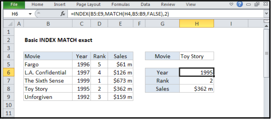
11. INDEX MATCH

INDEX MATCH is an improvement and advance alternative to the VLOOKUP formula. It’s a compelling combination of Microsoft Excel formulas that will make your financial work so easy.

The INDEX function returns the value of a cell in a table based on the column and row number.

MATCH formula returns the position of a cell in a row or column.

Original Formula : =INDEX(data,MATCH(value,column_lookup,column,FALSE),column)

Example of the formula :

This shows how to use INDEX-MATCH to get information from a table based on an exact match. In the example shown, the formula in CELL H6:

=INDEX(B5:E9,MATCH(H4,B5:B9,FALSE),2)
And this  returns 1995, the exact year the movie Toy Story was released.

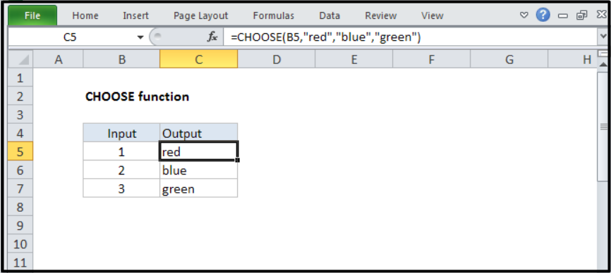
12. CHOOSE

For financial analysis, the CHOOSE function is a great tool. It allows to pick between a specific number of options and return the choice you’ve selected.

Original Formula:
=CHOOSE(index_num, value1, [value2], ….)

Example of the formula:

Microsoft Excel CHOOSE function returns a value from a list using a given index or position.
=CHOOSE(2,”red”,”blue”,”green”) gives back “blue”, as blue is the second value listed after the index number. The values provided to CHOOSE can include references.

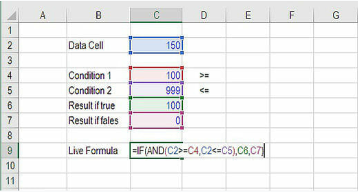
13. IF combined with AND/OR:

Combining IF condition with AND/OR can be a great way to efficient in various types of financial modes. If you’ve spent a significant deal of time can appreciate this formula more than anyone. 

Example of the formula:

=IF(AND(C2>=C4,C2<=C5),C6,C7) – As the number is between 100 and 999 the result is 100. You can also use text instead of a number. 

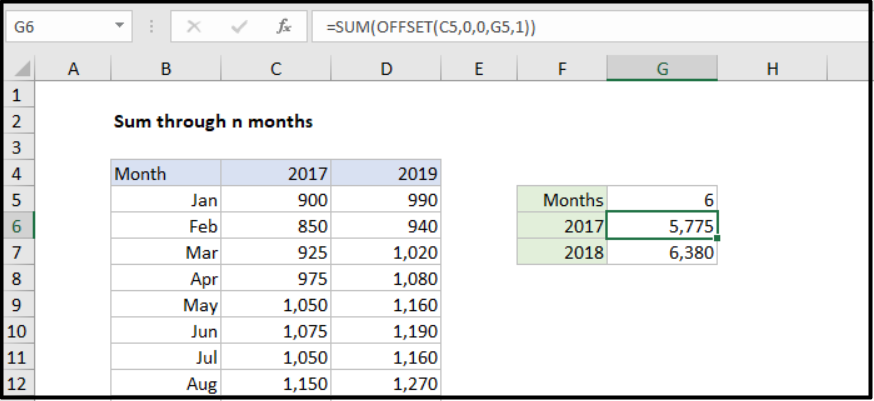
14. OFFSET combined with SUM or AVERAGE:

When the OFFSET function combined with other functions file SUM or average, you can create a pretty sophisticated formula. You can have more control over the SUM or AVERAGE function as you can set the cell numbers or make any alteration. With regular SUM formula, you’re limited to a static calculation, but buy adding OFFSET you can have cell reference move around.

Original formula:

=SUM(OFFSET(start,0,0,N,1))

To add a set of monthly data through n number of months, you can use a simple formula based on the SUM and OFFSET functions. In the example shown, the formula in G6 is:

=SUM(OFFSET(C5,0,0,G5,1))

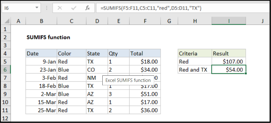
15. SUMIFS and COUNTIFS

These are great uses of conditional functions. SUMIF adds all the cells that meet specific criteria. And COUNTIF counts cells that meet a certain condition.

Original Formula:

=SUMIFS (sum_range, range1, criteria1, [range2], [criteria2], …)

Example of the formula:

In this example, SUMIFS is configured to sum values in column F when the color in column C is “red”. In the second example, SUMIFS is set to sum values in column F only when the color is “red” and the state is Texas (TX).

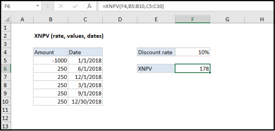
16. XNPV & XIRR

XNVP and XIRR allow you to apply specific dates to each cash flow that’s being discounted. So if you’re analyst working in investment banking, these formulas are lifesavers. 

There are some problems with Excel’s Basic formulas of IRR and NVP. These formulas assume the time periods between cash flows are equal. As an analyst, you’ll have many situations like when cash flows time period will not be the same. You can easily fix that problem with XNPV and XIRR.

The Microsoft Excel XNPV function calculates the net present value (NPV) of an investment based on a discount rate and a series of cash flows that occur at irregular intervals. 

Original Formula:
=XNVP(discount rate, cash flows, dates) 

Example of the formula:

=XNPV(F4,B5:B10,C5:C10)

XNPV doesn’t discount the initial cash flow. Usually, Subsequent payments are discounted based on a 365-day year. To discount to a specific valuation date, you can set up XNPV so that the first cashflow is zero, associated with the valuation date.

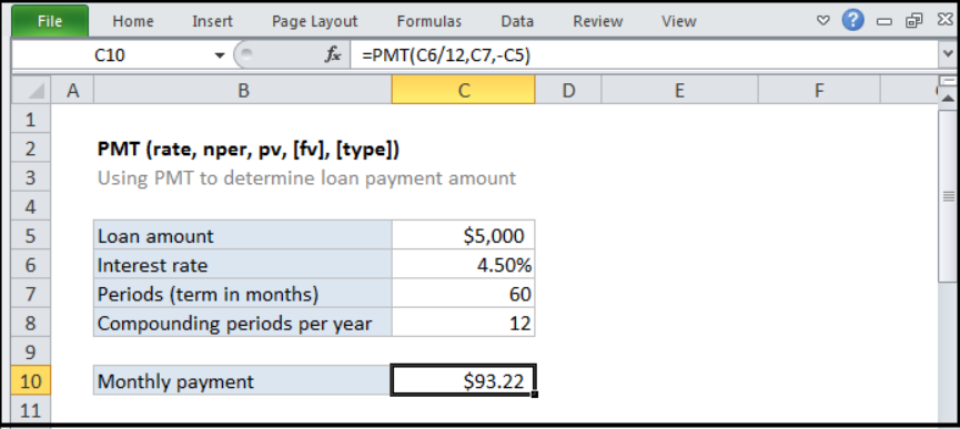
17. PMT & IPMT

The PMT formula is very powerful as it gives you the value of equal payments over the life of a loan. If you work in a commercial bank, real estate or any financial analyst position, you’ll understand these two formulas in details. 

This financial function returns the periodic payment for a loan. You can use the NPER function to figure out payments for a loan, given the loan amount, number of periods, and interest rate.

Original Formula :
=PMT(rate,nper,pv,[fv],[type])

• rate – The interest rate.
• nper – total number of payments.
• pv – total value of all loan payments now.
• fv – [optional] The future value
• type – [optional] When payments are due. 0 = end of period. 1 = beginning of period. Default is 0.

Example of the formula:

=PMT(C6/12,C7,-C5)
Calculates the monthly mortgage payment for a 5,000 mortgage at 4.5% for 30 years. Interest rate, periods and rate value are assigned accordingly to C6, C7, C5.

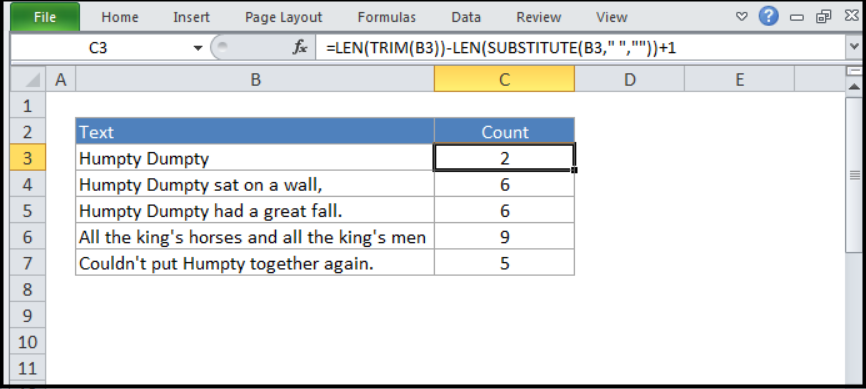
18. LEN & TRIM

These may be a little less common, but definitely very sophisticated formulas. LEN & TRIM formulas are great to those who need to organize and manipulate a large amount of data. It’s a shame that the data we get is not always perfect to work with. And sometimes there are more than one issues like extra spaces and the beginning or end of the cells.

This can come very handy to count words.
Original Formula :
=LEN(TRIM(A1))-LEN(SUBSTITUTE(A1, ” “, “”))+1

Example of the formula:
As you want to count the total words in a cell, you can use a formula based on the LEN and SUBSTITUTE functions. In this example, C3 contains this formula:
=LEN(TRIM(B3))-LEN(SUBSTITUTE(B3, ” “, “”))+1

We can see SUBSTITUTE removes all spaces from the text, then LEN calculates the length of the text without spaces. This number is then subtracted from the length of the text with spaces, and the number 1 is added to the final result, since the number of words is the number of spaces + 1.

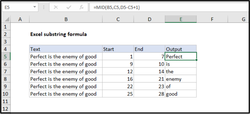
19. CELL, LEFT, RIGHT and MID functions 

These Excel functions can be combined to create some very powerful and complex formula to use. The CELL function can be very handy and can return a variety of information about the cell such as name, location, row, column and more. The LEFT function can return text from left to right.

Original formula :
MID(A1,start,end-start+1)
LEFT, RIGHT is similar.

Example of the formula:

In this example, we are using the MID function to extract text based on a start and end position. The MID function accepts three arguments: a text string, a starting position, and the number of characters to extract. The text comes from column B, and the starting position comes from column C.

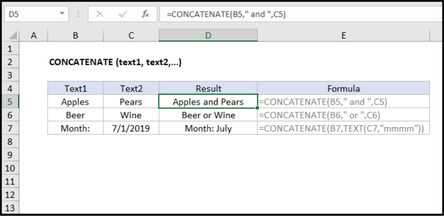
20. CONCATENATE

This is not a function but an innovative way of joining information from different cells and making worksheets more dynamic. This is an excellent tool for financial analysts performing financial modelling.

Original Formula:
=CONCATENATE (text1, text2, [text3],….)

Example of the formula:

The Microsoft Excel CONCATENATE function concatenates (joins) up to 30 text items together and returns the result as text. The CONCAT function replaces CONCATENATE in newer versions of Excel.

In the example shown, the following formula returns the string “Apples and Pears”:

=CONCATENATE(B5,” and “,C5) -returns the text “Apples and Pears”

These are the top 20 Microsoft Excel you should know to be more proficient in your office work and be a office guru!